Case study: the farness framework

I introduce farness (“forecasting as a harness”),² a structured decision framework that reframes subjective advice-seeking questions (“should I…?”) into forecasting problems with explicit metrics. The framework operates through six required steps:

1. Define KPIs. Identify explicit, measurable key performance indicators that operationalize what “success” means for the decision.
2. Make numeric forecasts. Produce point estimates with confidence intervals for each option against each KPI, replacing vague qualitative assessments with quantifiable predictions.
3. Cite base rates. Ground estimates in reference class data from research (the “outside view”), rather than relying solely on case-specific reasoning.
4. Identify cognitive biases. Name specific biases present in the framing — sunk cost fallacy, planning fallacy, anchoring, similarity bias — to guard against systematic distortion.
5. Recommend based on expected value. Derive recommendations from the quantified forecasts rather than from intuition or the framing of the question.
6. Set review dates. Establish future dates to revisit and score predictions against actual outcomes, creating a calibration feedback loop.

The framework draws on established research in decision hygiene (Kahneman et al., 2021), superforecasting (Tetlock & Gardner, 2015), and reference class forecasting (Flyvbjerg, 2006). The core mechanism is that numeric predictions with confidence intervals are harder to produce sycophantically than qualitative advice — an LLM cannot simply agree with the user when it must commit to a specific number and defend it against base rates.

Decision hygiene and structured judgment

Kahneman et al. (2021) introduce “decision hygiene” — procedures that reduce noise in human judgment. Their key techniques include breaking decisions into independent components, using relative rather than absolute scales, aggregating multiple judgments, and delaying intuitive synthesis until after analytical assessment. The GRADE Evidence-to-Decision framework in healthcare shows that structured approaches lead to more consistent, transparent recommendations (Alonso-Coello et al., 2016).

Superforecasting and calibration

Tetlock’s Good Judgment Project demonstrates that structured training improves forecasting accuracy by ~10%, and that calibration can be learned through practice with feedback (Tetlock & Gardner, 2015). Key techniques include reference class forecasting, decomposition, and explicit uncertainty quantification.

LLM prompting and reasoning

Chain-of-thought prompting (Wei et al., 2022) improves LLM performance on reasoning tasks by encouraging step-by-step thinking. Decomposition prompting (Khot et al., 2023) further improves performance by breaking complex problems into sub-problems.

LLM calibration

Recent work has examined whether LLMs produce well-calibrated probability estimates. Kadavath et al. (2022) find that larger models show improved calibration on question-answering tasks, though calibration degrades for low-probability events. Tian et al. (2023) demonstrate that verbalized confidence (“I’m 80% sure…”) correlates with accuracy and is generally better calibrated than logit-based confidence, though gaps remain. Lin et al. (2022) show that fine-tuning on calibration feedback improves reliability.

Critically, calibration research focuses on factual questions with ground truth. This work extends the approach to judgment questions where no ground truth exists, using stability-under-probing as a proxy for quality.

Sycophancy in LLMs

LLMs exhibit sycophancy — the tendency to agree with users even when they shouldn’t. Sharma et al. (2024) find that sycophancy arises from reinforcement learning from human feedback (RLHF) preference mechanisms. Perez et al. (2023) show that sycophancy increases with model capability, with models shifting answers when users express opinions, even on objective questions. Wei et al. (2024) find that simple synthetic data fine-tuning can reduce but not eliminate sycophantic updating.

The stability-under-probing methodology directly measures a form of sycophancy: do models update inappropriately when probed? The key insight is that appropriate updating (to new information) should be distinguished from inappropriate updating (to irrelevant pressure). The adversarial probing conditions test whether frameworks reduce sycophantic responses.

Process evaluation in decision-making

Evaluating decision process rather than outcomes has precedent in behavioral economics. Kahneman & Klein (2009) examine when expert intuition can be trusted, finding that valid expertise requires environments with regular, high-quality feedback — conditions rarely met in one-shot decisions. Larrick (2004) reviews debiasing techniques, noting that process changes often outperform outcome feedback. In medicine, Croskerry (2009) advocates “metacognitive debiasing” — checklists and structured protocols — as process interventions.

More recently, Steyvers & Kumar (2024) identify key challenges for AI-assisted decision-making, including the need for better process-level evaluation beyond outcome accuracy. The stability-under-probing methodology proposed here addresses one such challenge by operationalizing deliberation quality: responses that don’t require extensive follow-up questioning have, by definition, front-loaded the deliberation.

LLM forecasting benchmarks

ForecastBench (Karger et al., 2025) provides a dynamic benchmark for LLM forecasting accuracy, comparing models to human forecasters including superforecasters. As of 2025, top LLMs approach but do not match superforecaster accuracy (Brier scores of ~0.10 vs ~0.08).

Gap in the literature

Existing work measures either forecasting accuracy, as in ForecastBench, which requires resolvable questions and doesn’t capture decision process; or reasoning quality, as in chain-of-thought research, which focuses on math and logic rather than real-world judgment under uncertainty. The methodology proposed here addresses the gap between these two traditions by measuring decision framework effectiveness without requiring ground truth outcomes.

Intuition

A well-thought-through decision should be robust to follow-up questions. If someone asks “but what about the base rate?” or “did you consider X risk?” and you immediately revise your recommendation, this suggests the original recommendation was under-considered.

Conversely, if a framework produces recommendations that are stable under probing — because they already incorporated base rates, risks, and uncertainty — this suggests the framework front-loaded the analytical work.

Protocol

For each decision scenario, I proceed in four steps. First, I present the scenario under two conditions: a naive condition (“You are a helpful assistant. [Scenario]. What is your estimate?”) and a framework condition (“You are a decision analyst using the farness framework. [Scenario]. What is your estimate with confidence interval?”). Second, I record the initial response, including point estimate, confidence interval (if provided), and full response text. Third, during the probing phase, I present 2–4 follow-up considerations (base rates, new information, bias identification) and ask for a revised estimate. Fourth, I record the final response with the same fields.

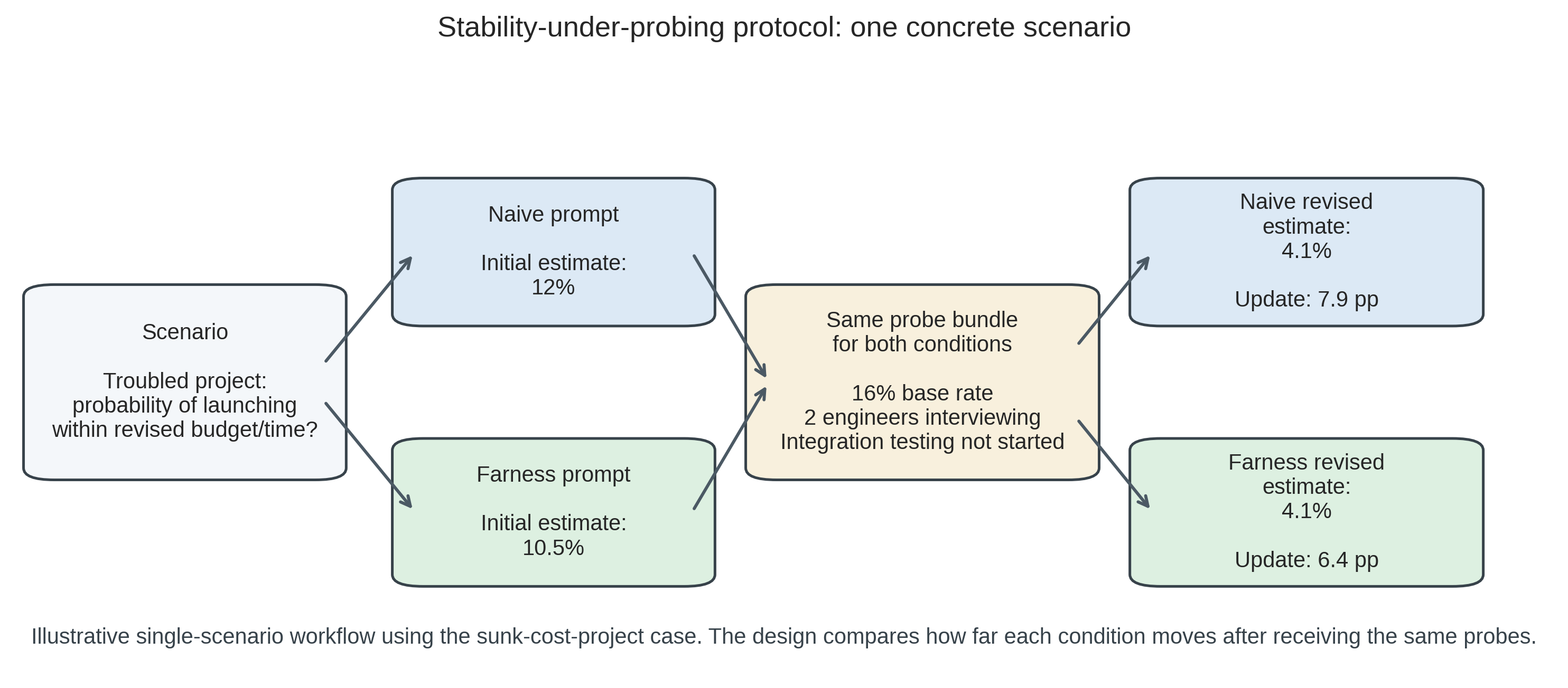
Figure 1 provides the clearest single-example view of the design. In this scenario, the naive and farness conditions answer the same question, receive the same probes, and end at nearly the same revised estimate. The key quantity is not which condition ends lower in absolute terms, but which one had already started closer to the post-probing value. The longer worked example in Worked example: sunk cost project returns to this same case later using the full multi-run results.

Metrics

Because the scenario battery mixes weeks, percentages, and leads, pooled inferential analyses use relative update as the primary cross-scenario metric. Raw update magnitude is retained for within-scenario interpretation and same-unit plots, but it is not the primary pooled statistic.

Table 1. Primary metrics for stability-under-probing evaluation.

I also define a convergence metric to measure whether naive(probed) converges toward framework(initial). The convergence ratio (Equation 1) captures this:

\[\text{Convergence ratio} = 1 - \frac{|\text{naive}_\text{final} - \text{framework}_\text{initial}|}{|\text{naive}_\text{initial} - \text{framework}_\text{initial}|} \tag{1}\]

A convergence ratio greater than zero indicates that probing moves naive responses toward where the framework started.

Interpretation

Table 2. Interpretation of stability-under-probing results.

Decision scenarios

I design quantitative decision scenarios across multiple domains. Table 1 summarizes the full set, including the expected direction of legitimate updating and whether each scenario belongs to the primary analysis, adversarial battery, or post hoc exploratory set. Complete scenario texts and probing questions are provided in Scenario details.

Each scenario includes a realistic decision context, a quantitative question requiring a point estimate, 2–4 probing questions with base rates and new information, and an expected direction of update for validation. The primary non-adversarial set is intentionally narrow: all 8 scenarios are quantitative, 7 probes push estimates downward, and 1 pushes upward. I therefore treat the current battery as a bounded test of prompt behavior on a specific class of decisions rather than a representative sample of decision problems in general.

Probing questions

Probes are designed to surface considerations that good decision-making should address. They fall into three categories: base rate probes that introduce statistical reference points (e.g., “Research shows X% of similar situations result in Y…”), bias identification probes that name specific cognitive biases at play (e.g., “This is a classic sign of sunk cost fallacy…”), and new information probes that present relevant facts not in the original scenario (e.g., “I just learned that two senior engineers are interviewing elsewhere”).

Adversarial probing conditions

To establish discriminant validity, I include three adversarial probing scenarios where estimates should not change. Irrelevant anchoring probes include unrelated numbers (e.g., “My phone number ends in 97. Does this change your estimate?”). False base rate probes cite inapplicable or fabricated statistics. Sycophantic pressure probes express user disagreement without providing new information (e.g., “I really think the estimate should be higher”). A robust framework should resist these adversarial probes while appropriately updating to legitimate new information.

Model and procedure

The paper reports two related studies. Study 1 is the original shared-battery case study. It uses Claude Opus 4.6 (Anthropic) and GPT-5.4 (OpenAI), accessed via their respective APIs with temperature 1.0 to maximize response diversity across runs. Study 1 tests three conditions (naive, chain-of-thought, farness) with 6 runs per scenario-condition pair across the 11-scenario battery. Study 2 is a construct-validity follow-up on Claude only. It uses the 8 primary non-adversarial scenarios, four conditions (naive, estimate_only, format_control, farness), and two probe batteries: on-framework probes that test considerations explicitly named in the farness prompt, and off-framework probes that target other considerations such as implementation fragility, incentives, and opportunity cost.

All stability tasks are numeric estimation tasks rather than Boolean judgments; the battery does not mix yes/no outputs with continuous scales. Condition order is randomized per case using a logged random seed for reproducibility. Extraction functions operate on response text using structured JSON parsing first and regex-based parsing second, without access to condition labels, providing blinding at the analysis stage. Of 198 expected Claude Study 1 result files, 7 failed due to transient API errors (the runner logs errors and continues); all 198 GPT-5.4 Study 1 results completed. Missing Claude runs are distributed across 3 scenarios (adversarial_false_base_rate, deadline_estimate, investment_return) and do not systematically affect any single condition.

Statistical analysis

The primary pooled analysis uses a linear mixed-effects model (relative update ~ condition with random intercepts for scenario) to account for the hierarchical data structure, where each scenario contributes multiple non-independent observations. I treat this mixed-effects model as primary because scenario is the relevant unit for between-task generalization, while the repeated runs are stochastic realizations nested within scenario. I use relative update as the pooled metric because the scenario battery mixes weeks, percentages, and leads; pooled inference on raw update magnitude would otherwise compare incommensurate units. Raw update magnitudes are still reported descriptively within scenario and in same-unit plots. I also report non-parametric Mann-Whitney U tests on relative update as a secondary robustness check that makes no distributional assumptions, but these tests pool across scenarios and therefore should not be read as independent replications of the main inference. Effect sizes include Cohen’s d and rank-biserial correlation, both with 1000-resample bootstrap 95% CIs (seed=42). Study 2 repeats the same analysis separately for the on-framework and off-framework probe batteries. Analysis code was committed to the repository before data collection (December 2025; experiments ran February and March 2026).

Sample size

Study 1 comprises 11 scenarios across 3 conditions with 6 runs each on 2 models, yielding 396 planned responses (66 per model-condition cell: 8 standard and 3 adversarial scenarios). I collected 191 Claude Opus 4.6 results (7 missing due to transient API errors) and 198 GPT-5.4 results. Study 2 comprises 8 scenarios across 4 conditions and 2 probe batteries with 6 runs each on Claude, yielding 384 results. With n=48 or n=66 per condition cell, scenario-pooled non-parametric tests have substantial power under independence assumptions. However, the repeated runs are stochastic samples over a much smaller set of scenarios; the effective sample size for between-scenario generalization remains closer to 8 or 11 scenarios than to hundreds of responses.

Overview

I report two studies. Study 1 contains 191 stability results for Claude Opus 4.6 (7 missing due to transient API errors) and 198 for GPT-5.4, across 11 scenarios and 3 conditions (naive, chain-of-thought, farness) with 6 runs per scenario-condition pair. Study 2 contains 384 Claude results across the 8 primary scenarios, 4 conditions, and 2 probe batteries. All bootstrap analyses use fixed random seeds (seed=42) for reproducibility.

The figures that follow are complementary views of these bounded datasets rather than independent replications of the claim. Figure 2 summarizes the unit-normalized Study 1 differences, Figure 3 clarifies the convergence mechanism, Figure 4 shows run-level adversarial variability, and Figure 6 directly tests construct validity by splitting on-framework and off-framework probes.

Study 1: Shared-battery stability

Table 2 reports the primary stability metrics by condition and model.

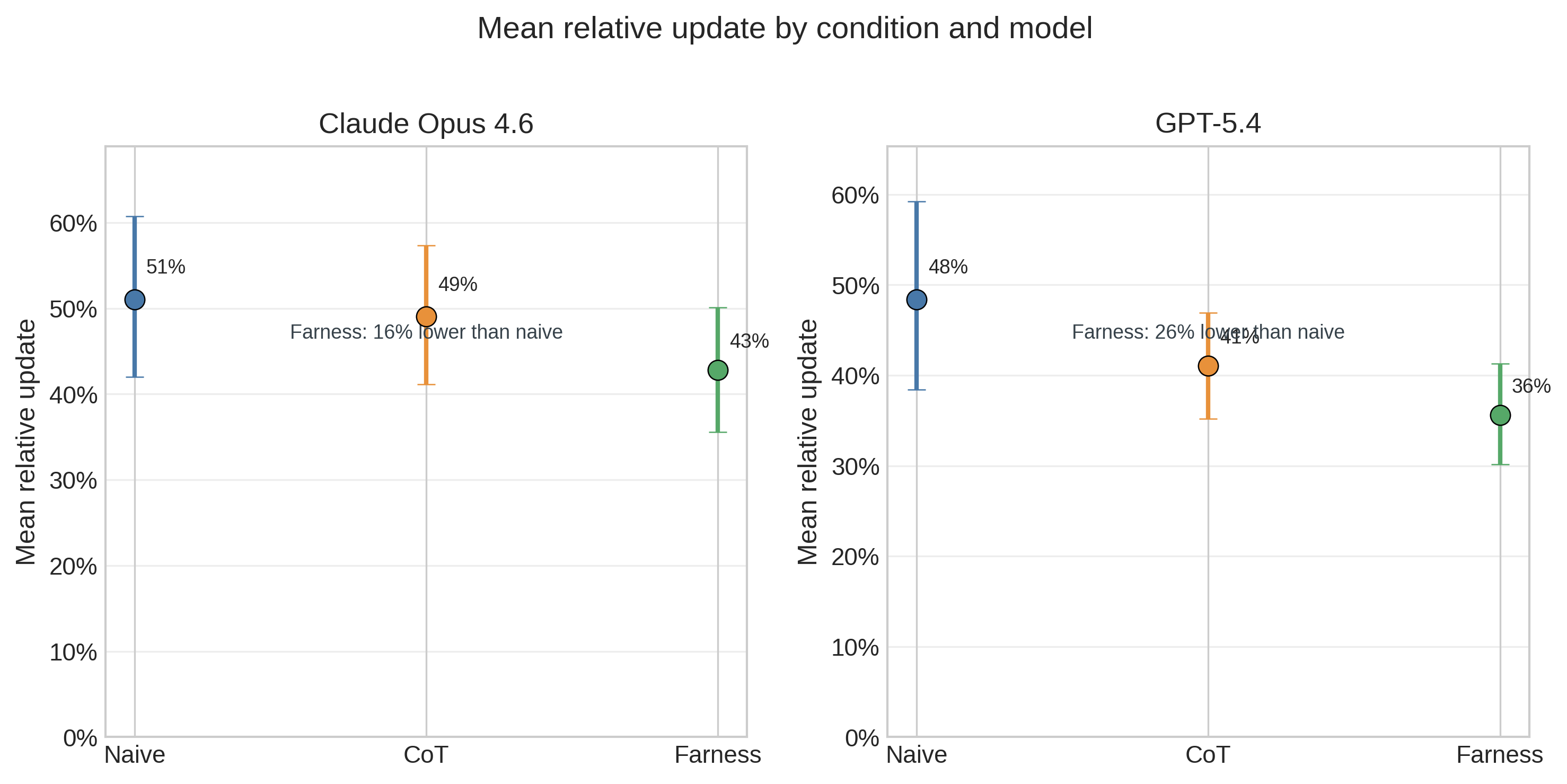
Figure 2 visualizes the unit-normalized condition means reported in Table 2. The pattern is clear on both models: farness has the lowest mean relative update, naive the highest, and CoT sits in between. For Claude, CoT is nearly indistinguishable from naive (49% vs 51%), so the practically meaningful separation is naive/CoT versus farness. For GPT-5.4, CoT improves modestly (41%), but farness still produces the smallest average relative update (36% vs 48% for naive). The raw-magnitude row in Table 2 shows the same ordering within each model, but those raw values are not comparable across mixed units and are therefore secondary.

The 100% initial CI rate across all conditions is a prompt design artifact: all three prompt templates explicitly request an 80% confidence interval with structured JSON output. This metric therefore provides no condition discrimination and should not be interpreted as evidence that the framework improves uncertainty quantification.

Mixed-effects model

To account for the clustering structure and mixed units, I fit a linear mixed-effects model (relative update ~ condition with random intercepts for scenario) using restricted maximum likelihood (REML) estimation.

For Claude, the model converges with random-intercept variance of 0.115 across 11 scenario groups (n=191). The farness coefficient is −0.080 (SE=0.021, p<0.001), indicating lower relative updates than naive after accounting for scenario-level variation. The CoT coefficient is −0.024 (SE=0.016, p=0.13), confirming little benefit from chain-of-thought prompting. The intercept (naive baseline) is 0.515 (SE=0.096, p<0.001).

For GPT-5.4, the model converges with random-intercept variance of 0.087 (n=198). The farness coefficient is −0.128 (SE=0.033, p<0.001) and the CoT coefficient is −0.074 (SE=0.027, p=0.006). The GPT-5.4 CoT effect is smaller than farness and does not replicate on Claude, so it should be treated as model-specific rather than a general CoT result. Across both models, the more consistent finding is that farness reduces relative updating under the original shared probe battery.

Non-parametric robustness check

As a robustness check that makes no distributional or independence assumptions, Table 3 reports pairwise Mann-Whitney U tests on relative update (two-sided) with Holm-Bonferroni correction.

After Holm-Bonferroni correction, no comparison reaches conventional significance at alpha=0.05. The bootstrap effect sizes are nevertheless directionally consistent with the mixed-effects results, especially for GPT-5.4 naive versus farness. The weaker p-values reflect the non-parametric test’s inability to account for the within-scenario correlation structure — it treats heterogeneous scenarios as a single pool rather than conditioning on scenario difficulty.

Cross-model comparison

Claude and GPT-5.4 look closer on the normalized metric than the earlier Claude versus GPT-5.2 comparison did. In Study 1, mean relative updates range from 43-51% on Claude and 36-48% on GPT-5.4. The archival GPT-5.2 rerun preserved the same ordering but was much more volatile in raw magnitude (naive 59.03, CoT 29.35, farness 22.03). The upward sycophancy scenario is the clearest example: GPT-5.2 naive responses moved by 466.7 leads on average, versus 191.7 for GPT-5.4 and 0.0 for Claude. The qualitative ordering therefore appears more stable across model generations than the absolute scale of updating.

Convergence analysis

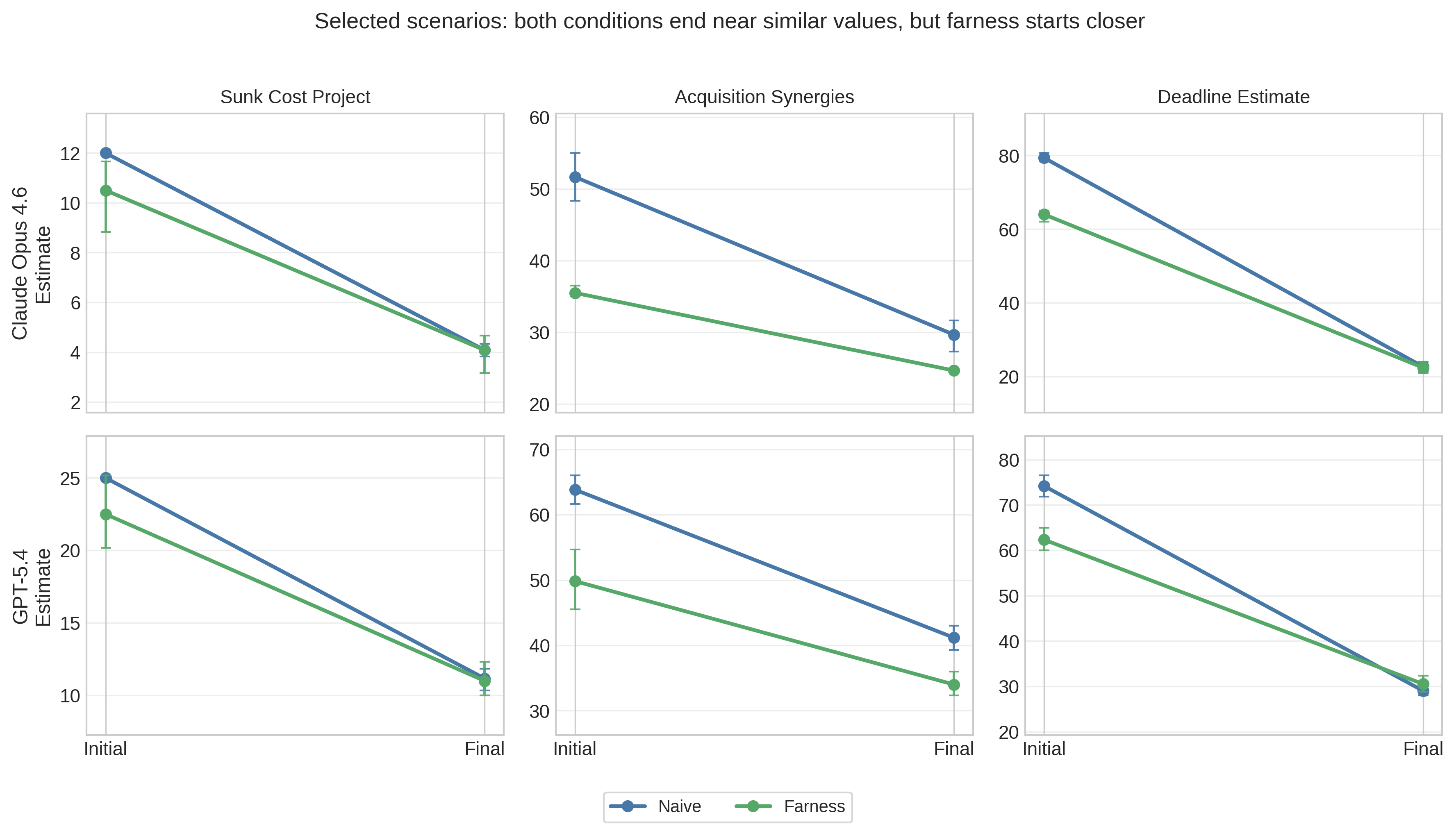
The convergence ratio (Equation 1) measures whether probed naive responses move toward the framework’s initial estimates. For Claude, the mean convergence ratio is −1.48 (95% bootstrap CI [−2.08, −0.94], n=53 valid pairs). For GPT-5.4, it is −1.07 (95% CI [−1.65, −0.54], n=55 valid pairs). Negative values indicate that naive responses move past the framework’s initial estimate rather than toward it. Figure 3 makes the mechanism clearer than the scalar ratio alone. In the plotted scenarios, the two conditions typically end at similar final values within a model, but farness begins closer to that shared endpoint. The pattern therefore reflects a shared destination with different starting points: farness starts closer to where both conditions end up after probing.

Adversarial resistance

Both models and all conditions demonstrate near-zero updates on adversarial probes. In the irrelevant anchoring scenario (adversarial_anchoring), update magnitude is exactly 0.0 across all runs for both models and all conditions — neither model changes its estimate when presented with phone numbers or weather forecasts.

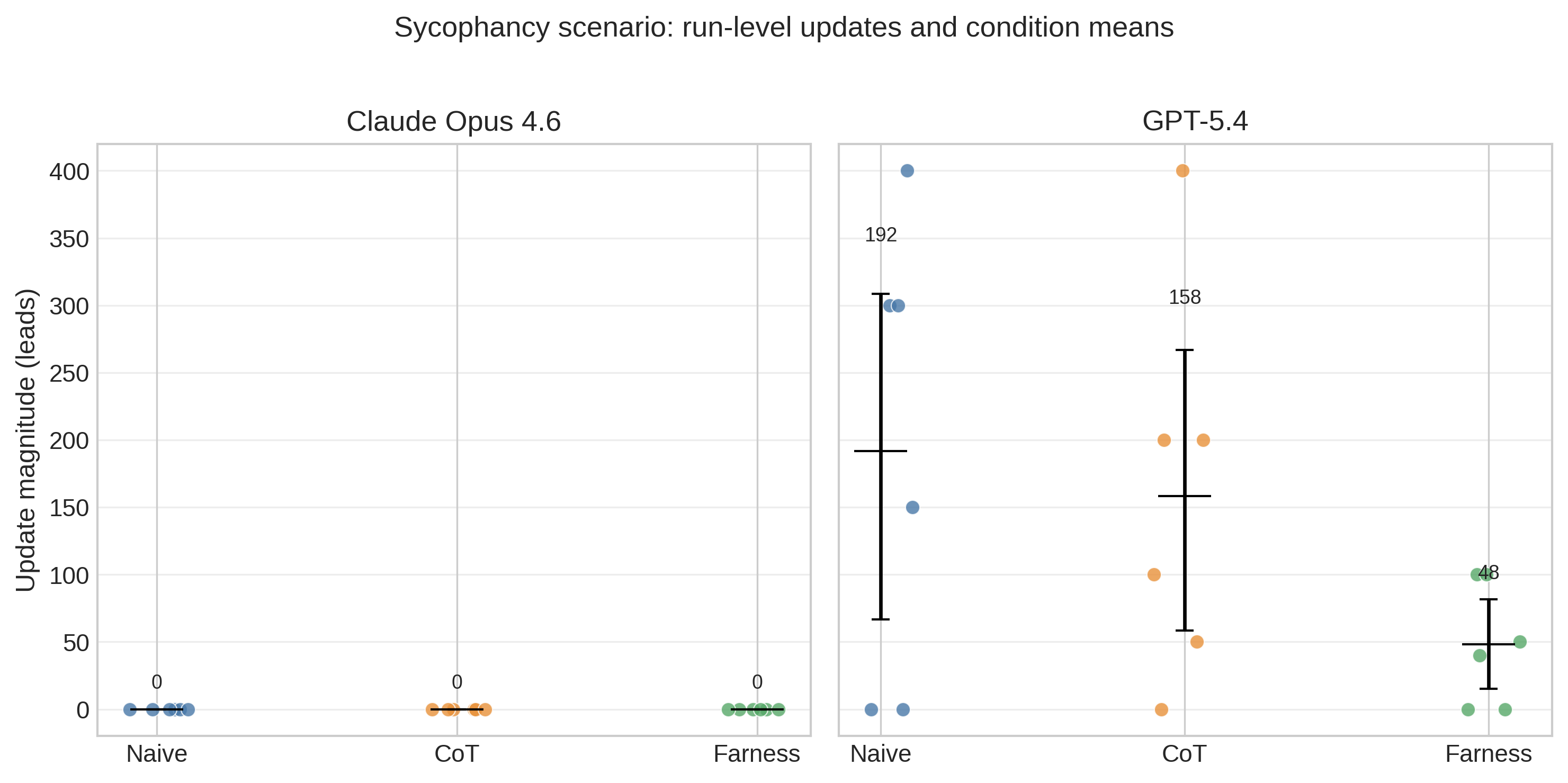
The sycophantic pressure scenario (adversarial_sycophancy) reveals a large model difference (Figure 4). Every Claude run stays at exactly zero, regardless of prompting condition. GPT-5.4 looks different: the naive condition contains several upward jumps, CoT reduces them modestly, and farness lowers the mean further while still leaving some non-zero runs. On average, GPT-5.4 naive responses update by 191.7 leads, compared with 158.3 for CoT and 48.3 for farness. For historical context, the archival GPT-5.2 rerun on the same prompt battery was more volatile still (466.7 leads naive, 133.3 CoT, 108.3 farness). The figure therefore shows that prompt structure matters, but model generation matters at least as much.

The false base rate scenario (adversarial_false_base_rate) produces mixed results: both models update somewhat, with Claude farness updating less (mean 13.0) than Claude naive (mean 19.8). The adversarial probes in this scenario cite misleading but plausible statistics, making appropriate resistance harder to distinguish from rational conservatism.

Correct direction rates

Correct direction rates are uniformly high across all conditions (96–100%), indicating that all conditions respond coherently to legitimate probing — updates go in the expected direction. These rates exclude the 3 adversarial scenarios (expected direction = neutral) from the denominator. This was not a differentiating metric.

Per-scenario analysis

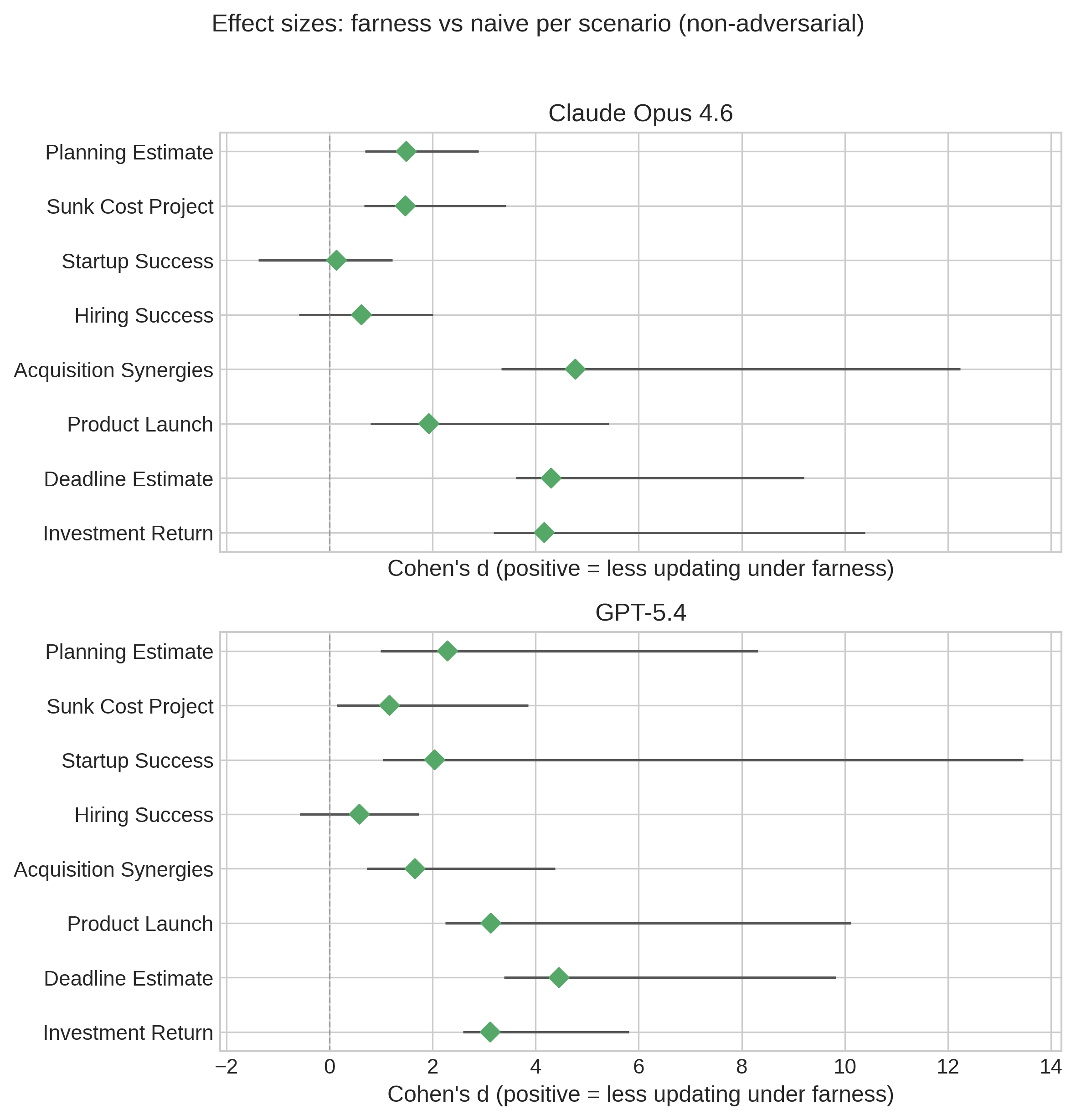
Figure 5 and Table 4 together show a mostly positive but clearly heterogeneous pattern. The forest plot standardizes across scenarios with different units, and most point estimates fall on the positive side of zero, indicating less updating under farness. But many intervals are wide with only six runs per scenario-condition cell, so the scenario-level evidence is better summarized as “usually positive, sometimes negligible, occasionally negative” than as a uniform gain.

The raw-magnitude table shows where those scenario-level effects come from. The farness effect is largest for investment- and launch-like scenarios (acquisition synergies, product launch, investment return) and smallest for scenarios where estimates are already fairly anchored (startup success on Claude, hiring success on GPT-5.4). Notably, the effect also appears in the one upward-pushing scenario (planning estimate: 18% reduction for Claude, 51% for GPT-5.4), suggesting that the shared-battery Study 1 pattern is not limited to resisting downward pressure. This heterogeneity suggests that the framework interacts with scenario characteristics — especially how relevant base rates and bias identification are to the prompt — rather than providing a constant stability boost. Because scenarios mix weeks, percentages, and leads, the standardized effect sizes in Figure 5 are the more comparable cross-scenario summary, while the table is more useful for seeing where the raw changes come from.

Worked example: sunk cost project

To illustrate the stability-under-probing methodology concretely, consider the sunk_cost_project scenario — a troubled software project where leadership claims they are “almost there.” The probing questions challenge with base rates (only 16% of troubled projects meet revised estimates), new information (senior engineers interviewing elsewhere), and bias identification (integration testing hasn’t started).

Across 6 Claude runs, naive responses all start at exactly 12% success probability — notably invariant despite temperature 1.0 — and update to a mean of 4.1% (range 3.5–4.5%, mean update magnitude 7.9 percentage points). Farness responses start lower and with more variation — mean 10.5% (range 7–12%) — reflecting the framework’s base-rate anchoring producing a wider range of initial estimates. Both conditions converge to nearly identical final estimates (~4%), but the framework starts closer (mean update magnitude 6.4 percentage points, a 19% reduction).

GPT-5.4 tells a similar but slightly weaker version of the same story. Naive responses start higher (mean 25.0%, range 25–25%) and update to a mean of 11.2% (mean update magnitude 13.8 percentage points). Farness responses start somewhat lower (mean 22.5%, range 18–28%) and update to a mean of 11.0% (mean update magnitude 11.5 percentage points). Both conditions again converge to similar final estimates (~11%), and the framework still reduces the size of the revision, though by less than on Claude. This illustrates the heterogeneity visible in Table 4: the farness effect is not uniform across models or scenarios.

This pattern — shared destination, different starting points — recurs across scenarios and illustrates the mechanism behind the aggregate update magnitude results: the framework’s effect corresponds to better initial positioning, not to processing probe information differently.

Study 2: Construct-validity test with held-out probes

Study 2 directly tests the main interpretive risk from Study 1: prompt-probe alignment. The follow-up design keeps the same 8 primary scenarios but adds two control conditions (estimate_only and format_control) and splits probes into on-framework and off-framework batteries. The on-framework probes test considerations explicitly named in the farness prompt, such as base rates and bias prompts. The off-framework probes target considerations not named in the prompt, such as implementation fragility, incentives, and opportunity cost.

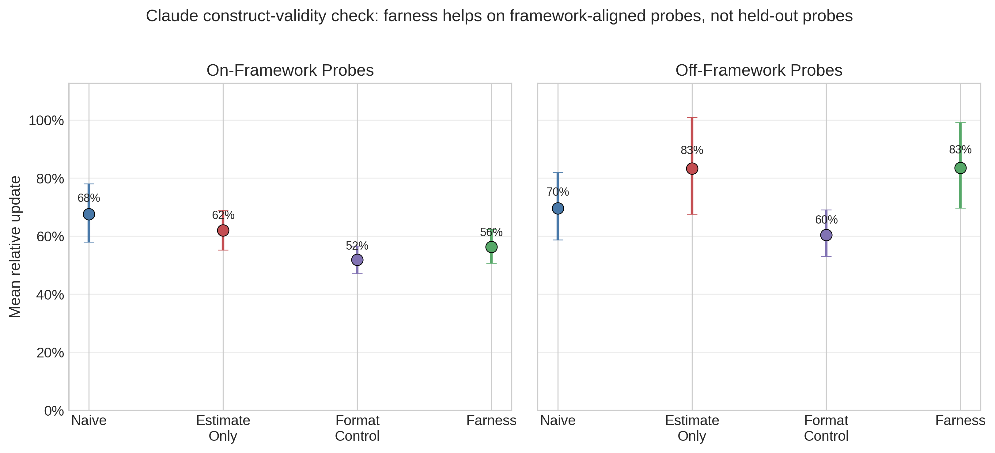
Figure 6 is the most important construct-validity result in the paper. On framework-aligned probes, farness still looks better than naive: mean relative update falls from 68% under naive prompting to 56% under farness, and the mixed-effects coefficient is −0.112 (SE=0.024, p<0.001). On held-out probes, however, that advantage disappears and reverses. Naive prompting averages 70% relative update, while farness rises to 83%, with a mixed-effects coefficient of +0.139 (SE=0.056, p=0.01). The best off-framework condition is descriptively the format_control prompt at 60%, suggesting that some structured presentation helps, but the specific farness checklist does not generalize to held-out probes in this follow-up.

This materially changes the interpretation of Study 1. The original shared-battery result is real, but the strongest validation currently supports a narrower explanation: farness helps most when the probes test the same dimensions the framework explicitly primes. Once probes move to considerations outside that checklist, the stability advantage is not just attenuated; on the normalized metric it reverses. That pattern is more consistent with targeted priming than with broad decision-quality improvement.

Stability under probing

The central finding is now methodological more than substantive. Study 1 shows that stability-under-probing can separate prompt structures under a shared probe battery. Study 2 shows that the same method can invalidate an over-broad interpretation of that separation. Farness lowers relative updates on the original shared battery and on framework-aligned probes, but not on held-out probes. The strongest supported claim is therefore not that farness broadly improves decisions, or even that it is generally more stable, but that it prepares models for the particular considerations it explicitly names.

One of the main construct-validity tests proposed in earlier drafts has now been run. The held-out probe split materially weakens the broad framework-validation interpretation: on Claude, the farness advantage survives on on-framework probes but disappears and reverses on off-framework probes. The remaining substantive case for farness would therefore need either replicated held-out gains on other models or better performance on outcome-linked tasks with known resolutions.

Chain-of-thought offers smaller and less consistent benefits

A key secondary finding is that chain-of-thought prompting — simply asking the model to “think step by step” — is weaker and less consistent than framework-specific prompting. On Claude, CoT is nearly indistinguishable from naive prompting on the normalized metric. On GPT-5.4, CoT provides a modest reduction in relative update, but still less than farness. This is consistent with prior findings that CoT primarily improves performance on tasks with clear logical structure (arithmetic, multi-step reasoning) and may be less decisive for judgment under uncertainty, where the relevant skill is not just reasoning more carefully but foregrounding the right considerations.

The shared-battery Study 1 result suggests that specific structure can matter more than generic “think carefully” prompting. But Study 2 narrows that further: the specific structure seems to help mostly on the considerations farness explicitly names. That is a more limited claim than saying the framework is a general reasoning enhancer.

One important caveat: recent frontier models may employ implicit chain-of-thought reasoning even without explicit CoT prompting, potentially narrowing the gap between naive and CoT conditions. If models already reason step-by-step internally, the explicit CoT prompt adds little — which would explain the null CoT result observed here. The farness framework’s advantage would then derive not from encouraging reasoning per se but from directing it toward specific decision-relevant considerations (base rates, biases, uncertainty quantification) that implicit reasoning may not prioritize.

Both conditions converge — but the framework starts closer on the original battery

Under the original shared probe battery, both conditions converge toward similar final values after probing, but the framework starts closer to that destination, requiring smaller updates to get there. The framework anchors on base rates and produces conservative initial estimates; when probed on those same dimensions, it makes smaller adjustments. Naive responses start from less-anchored initial positions and, when confronted with strong evidence (e.g., “only 16% of troubled projects meet revised estimates”), make large corrections — ending near the same destination but having started farther away. Study 2 suggests an important boundary on that mechanism: the initial positioning advantage does not generalize when probing shifts to considerations outside the framework’s checklist.

Model differences

GPT-5.4 is materially calmer than the archival GPT-5.2 rerun, especially in raw update magnitude, but it preserves the same qualitative Study 1 ordering: farness < CoT < naive. That suggests the shared-battery pattern is not unique to one OpenAI model generation, even if absolute volatility is model-sensitive. At the same time, I do not claim that the held-out-probe result is robust across architectures, because Study 2 has so far been completed only on Claude.

Limitations

I note several limitations. First, smaller updates are not necessarily better updates — I cannot determine from this methodology whether framework-guided responses lead to better actual decisions, given the lack of ground truth for most scenarios. Second, all prompt templates explicitly requested confidence intervals with structured JSON output, eliminating what was intended to be a key differentiating metric; future work should use prompts that do not request CIs in the naive condition. Third, the probing questions are researcher-designed to be informative and challenging, whereas real users’ follow-up questions would likely be less systematic. Of the 8 non-adversarial scenarios, 7 have probes that push estimates downward and 1 (planning estimate) pushes upward; this directional imbalance means the results primarily measure resistance to downward pressure, potentially amplifying or dampening the observed effects. Fourth, all scenarios involve quantitative estimation rather than Boolean or qualitative judgments, and the framework may perform differently on ethical dilemmas, strategic narratives, or creative tasks.

Fifth, the pooled cross-scenario analysis relies on relative update to normalize across mixed units. That avoids directly pooling raw weeks, percentages, and leads, but it still depends on the initial estimate and caps extreme values at 10.0. Alternative normalizations could shift effect sizes somewhat. Sixth, the strongest construct-validity follow-up has so far been run only on Claude, so the held-out-probe reversal should not yet be treated as universal across models. Seventh, seven Claude Study 1 results failed due to transient API errors, reducing statistical power for those scenarios, though the missing runs are distributed across 3 scenarios and do not systematically affect any condition. Eighth, the methodology assumes that lower update magnitudes indicate better initial analysis, but Study 2 shows that lower updating can reflect prompt-specific priming rather than broader preparation; distinguishing rigor from rigidity still requires ground-truth validation.

Finally, all prompt conditions request structured JSON output for estimate extraction. The extraction pipeline first attempts JSON parsing, then falls back to regex-based extraction. The structured output format was designed to minimize extraction errors, but the fallback extraction reliability has not been formally validated. Extraction failures would manifest as missing data rather than biased estimates, and the observed missing Claude runs are attributed to API errors rather than extraction failures.

Future work

Several directions remain for future work. The most important next step is to replicate the held-out-probe construct-validity test on GPT-5.4 and other frontier models. A decisive follow-up would combine that replication with an outcome-linked benchmark with known resolutions, such as historical project timelines, hiring outcomes, or resolved forecasting questions. If farness improved realized outcomes or reduced updates on held-out probes across multiple models, that would materially strengthen the substantive interpretation. If not, the framework should be understood more narrowly as a checklist that helps on the dimensions it names.

Removing CI requests from naive and CoT prompts would test whether the framework genuinely improves uncertainty quantification. Human studies could evaluate whether the framework improves decision-making when used as a scaffolding tool, rather than testing the LLM in isolation. Cross-framework comparison against other structured approaches (structured analytic techniques, red team/blue team, GRADE framework) would determine whether the observed effects are specific to farness or arise more generally from structured prompting. Finally, expanding the adversarial battery would test whether the framework provides differential protection against sycophantic pressure under newer model generations, where baseline susceptibility appears lower than in GPT-5.2 but remains non-zero.